When asked what embedding model and similarity metric they’ve used, most people answer something like: “OpenAI embeddings with cosine similarity.”
That’s a perfectly valid answer. But it leads to deeper questions:
- What if you’re working with an open-source embedding model like BERT-base or MiniLM-base? Can you still use cosine similarity?
- What if you come across code that’s using Euclidean distance with OpenAI embeddings — is that wrong?
- Are there scenarios where Euclidean distance is actually better?
- Do recommendation systems have different considerations than RAG systems?
These were some of the questions we dug into in our team learning session last Friday. Let’s walk through the key takeaways.
First: the difference between Euclidean distance and cosine similarity
At a glance both compare vectors, but they focus on different things:
- Euclidean distance: compares the endpoints of the vectors. It’s the straight-line distance between two points.
- Cosine similarity: compares the directions. It measures the angle between vectors, ignoring how long they are.
Euclidean distance
For simplicity’s sake, let’s take two vectors 

Matematically:

This makes it clear why length matters here: even if two vectors point in almost the same direction, if one is much longer, the distance between their endpoints will still be large.

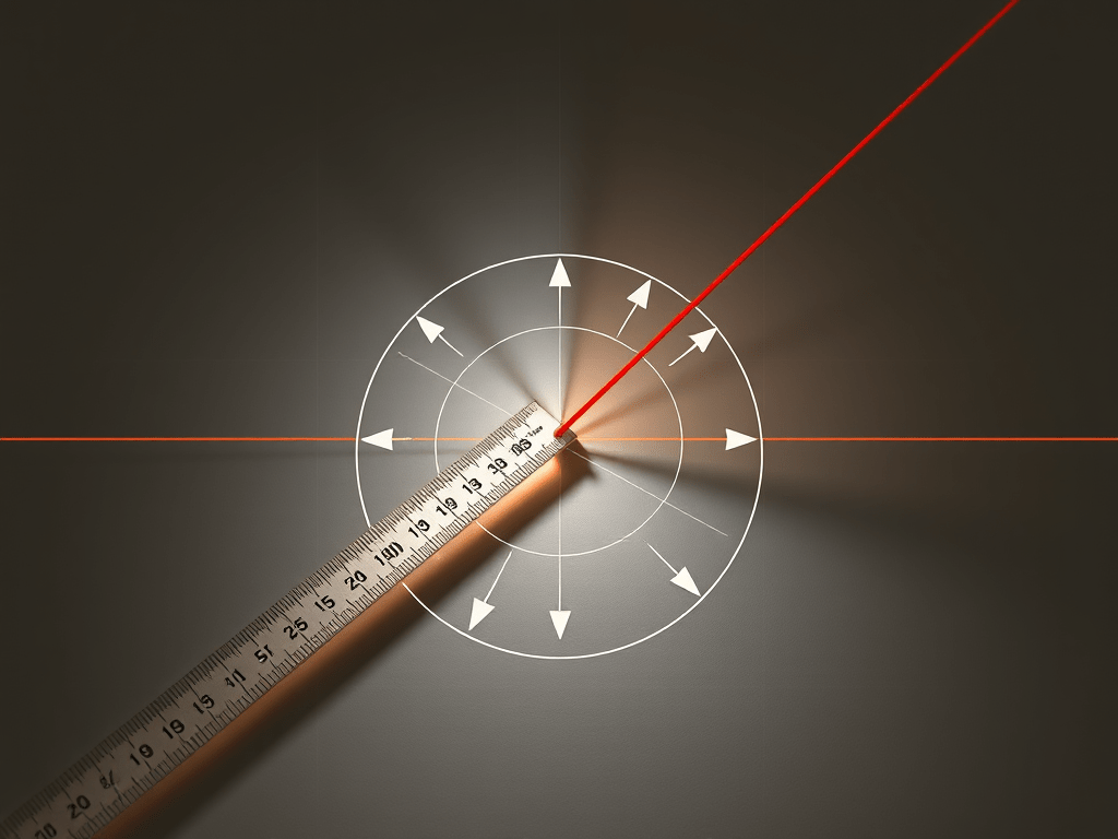
Cosine similarity
While Euclidean distance looks at the endpoints of vectors, cosine similarity only looks at their direction. Imagine projecting every vector onto the unit circle: cosine measures how close those directions are, regardless of how long the arrows are.
Mathematically:

Here 


- If the angle is 0° (vectors point the same way), cosine = 1 → perfectly similar.
- If the angle is 90° (orthogonal), cosine = 0 → no similarity.
- If the angle is 180° (opposite directions), cosine = –1 → maximally dissimilar.
Visually: even if one arrow is much longer, if they point in the same direction their cosine similarity is still 1.

The intuition with three vectors
Imagine three vectors: A, B, and C:

- As you can see, B is more aligned in direction with A than C is.
- With Euclidean distance, A–C (~ 9.2) looks closer than A–B (~ 13.5) because C’s tip is nearer to A’s tip, even though the angles are different.
- With cosine similarity, A–B wins, because alignment (angle) matters more than raw length.
This is exactly the situation where Euclidean and cosine will disagree on ordering. So, this is why you need to be mindful of your choice of the comparison metric.
Why normalization matters
A common trick is to normalize vectors so their length is 1 (i.e., put them on the unit circle or unit sphere). The math looks like this:

Basically, take the vector 
When both vectors are normalized, this distance is just another way of measuring the angle between them — which is exactly what cosine similarity does.

So, in our example, after normalization B is closest to A, followed by C – with both cosine similarity and Euclidean distance.
OpenAI embeddings already come normalized. Even though most people use cosine similarity without a second thought, even if you use Euclidean distance with them, you’ll get the same neighbors as cosine similarity — the rankings are identical.
When magnitude matters: why not always normalize?
It’s tempting to think you should always normalize embeddings and stick to cosine similarity. After all, that’s what most semantic search and RAG systems do. But normalization isn’t always the right move, because sometimes the magnitude of the embedding carries meaning.
Remember, the dot product between two vectors is:

That means it encodes both alignment (the angle) and magnitude (the length of each vector). If length itself encodes a signal you care about, dot product or Euclidean distance can be the right tool, while cosine would wash that information away.
Examples:
- Number of views on a video – a 10,000-view video might need to be treated differently from a 100-view video, even if the content is otherwise identical.
- Price of an item – if embeddings include “price” as one axis, Euclidean distance will reflect a real dollar gap ($499 vs. $1,999), not just semantic similarity.
- Quantity sold / demand – embeddings that include sales volume should allow high-demand items to naturally stand apart from slow movers.
- User activity level in recommendations – in collaborative filtering systems, highly active users often have embeddings with larger norms. Dot product/Euclidean distance naturally lets that popularity signal influence similarity scores.
In practice, large-scale recommendation systems have successfully leveraged this property. For example, Yahoo’s Prod2Vec approach (Grbovic et al., 2015) applied Word2Vec-style training to user interaction sequences. They found that the resulting embeddings captured not only “semantic” relations between products, but also popularity and frequency effects in the vector norms which were signals that were directly useful for recommendations.
So, you might think: does this mean I don’t have to worry about Euclidean or dot product in RAG systems? The answer is: usually not. But, here’s the fun part: most vector databases (FAISS, Pinecone, Weaviate, Milvus, etc.) implement cosine similarity by normalizing embeddings once and then using dot product internally. Why dot product? Because once embeddings are normalized, dot product works the same for ranking as Euclidean, but is faster to compute.
My own small experiment, described below, confirmed this: Dot product was slightly faster than Euclidean on normalized embeddings (~1.1× speedup in my run), since it’s just multiply-and-sum with no subtractions/squares.
After normalization, cosine and Euclidean gave identical nearest-neighbor rankings.
THE Experiment
- Generated ~20,000 database vectors and 200 query vectors with an embedding size of 384 (roughly what you’d get from MiniLM).
- For each query, retrieved the top-K neighbors using:
- Dot product (cosine if vectors are normalized)
- Squared Euclidean distance
Tested both on raw vectors and on normalized vectors (so that 
Results:
- On normalized vectors, cosine and Euclidean produced identical neighbor rankings.
- In terms of performance, dot product was about 1.1× faster than Euclidean on normalized embeddings. That’s because dot product is just multiply-and-sum:
While squared Euclidean requires subtracting, squaring, and adding:
So Euclidean does more work per dimension, even if the final square root is skipped. - On raw (unnormalized) vectors, Euclidean and cosine gave different rankings, because vector length influences Euclidean distance but is canceled out in cosine.


Takeaways from the experiment:
- After normalization, dot product, cosine, and Euclidean distance are effectively the same in terms of ranking.
- Dot product is slightly faster in practice which explains why most vector databases implement cosine as “normalize once, then use dot product.”
- Before normalization, you can get very different results. Euclidean reflects both angle and magnitude, while cosine reflects only angle.
Recommendation vs. RAG systems
- In RAG systems, you care primarily about semantic similarity. Normalization is almost always what you want, so cosine (or normalized Euclidean) is the default.
- In recommendation systems, embeddings often mix semantic and behavioral signals. Magnitude might encode popularity, confidence, or frequency. In this world, dot product or Euclidean without normalization can be useful.
Decision Tree: When to Use Which

Key Takeaways
- Cosine similarity: great when direction = meaning; normalization removes scale.
- Euclidean distance: great when raw magnitudes carry interpretable meaning.
- Normalization: turns Euclidean into cosine for ranking purposes.
- OpenAI embeddings: already normalized, so Euclidean and cosine rank the same.
- Good rule of thumb in selecting the best similarity metric: match it to the one used to train your embedding model.
- Recommendations vs RAG: recommendations often want magnitude, RAG almost never does.

Leave a comment